
"Some questions don't want a number — they want a decision. Yes or no? This or that? That's where logistic regression shines."
Learning Objectives
By the end of this module, you will be able to:
- Explain how logistic regression differs from linear regression
- Understand how the "sigmoid" turns any number into a probability
- Tell apart binary, multinomial, and ordinal classification
- Understand why categories must be turned into numbers first
- Read a confusion matrix to judge a classifier
1. From "How Much?" to "Which One?"
In the last module, regression answered how much? with a number. But many real questions want a category instead:
- Is this email spam — yes or no?
- Is this tumor benign or malignant?
- Is this pumpkin orange 🎃 or white 👻?
That last one is our example. White pumpkins are sometimes called "ghost" pumpkins, so our question becomes delightfully simple: ghost, or not ghost?
Despite its name, logistic regression is really a classification tool. Here's the key visual difference from linear regression:
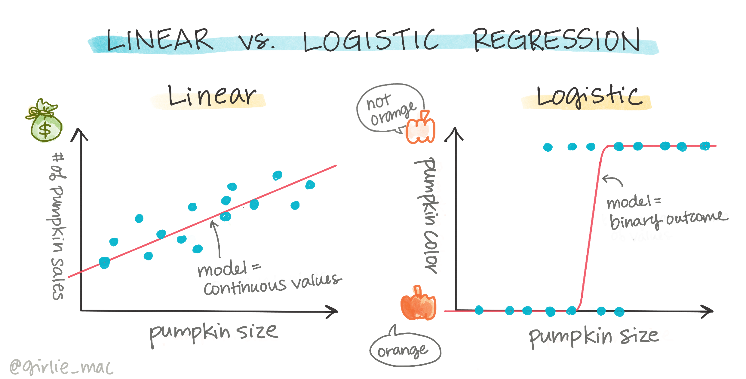
Concept: Linear regression draws a line that keeps going up forever (predicting amounts). Logistic regression bends that line into an S-shape that levels off between 0 and 1 — perfect for answering yes/no questions as a probability.
2. The Sigmoid: Turning Anything Into a Probability
The magic ingredient is the sigmoid function — an S-shaped curve that takes any number, however big or small, and gently squashes it into a value between 0 and 1.
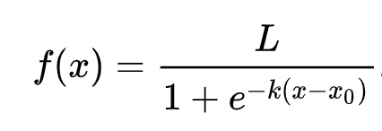
Why is that useful? Because a number between 0 and 1 is a probability. If the model outputs 0.92 for "is this a ghost pumpkin?", that's a confident yes. If it outputs 0.10, that's a confident no. We usually draw the line at 0.5: above it, we say "yes"; below it, "no."
Concept: The sigmoid is the bridge between the world of endless numbers and the world of yes/no decisions. It converts a raw score into "how likely is this?" — and that's exactly what a classifier needs.
3. Three Flavors of Classification
Logistic regression comes in three varieties, depending on how many categories you're choosing between:
| Type | Choices | Example |
|---|---|---|
| Binary | Exactly two | Ghost or not ghost; spam or not spam |
| Multinomial | Three or more, no order | Orange, White, or Striped |
| Ordinal | Ordered categories | Pumpkin size: mini < small < medium < large |
Did You Know? Unlike linear regression — which loved strongly correlated inputs — logistic regression is far more relaxed. Its input features don't need to be neatly correlated with each other, which makes it a friendly, forgiving first classifier for messy real-world data.
4. Machines Need Numbers: Encoding Categories
Here's a snag. Our pumpkin data is full of words: "Baltimore," "pie type," "orange." But machine learning algorithms only understand numbers. So before training, we translate categories into numbers — a step called encoding.
There are two friendly ways to do it:
- Ordinal encoding — for categories that have a natural order. Sizes become mini=0, small=1, medium=2, and so on, preserving the ranking.
- One-hot encoding — for categories with no order (like city names). Each option becomes its own yes/no column, so the model never wrongly assumes "Boston > Baltimore."
Pro Tip: Choosing the right encoding matters. Use ordinal only when order genuinely means something (sizes, ratings). For everything else — colors, cities, names — reach for one-hot so you don't invent a fake ranking the model will take seriously.
5. Building One in Practice
Just like every model in this track, it follows the same fit / predict rhythm — only the model's name changes:
[object Object], sklearn.linear_model ,[object Object], LogisticRegression

model = LogisticRegression()     ,[object Object],
model.fit(X_train, y_train)      ,[object Object],
prediction = model.predict(X_test)   ,[object Object],
Notice how little the code changes from Module 4's regression example. That consistency is the whole point of Scikit-learn — learn the pattern once, apply it everywhere.
6. Was It Right? The Confusion Matrix
To judge a classifier, we line up its guesses against reality in a little grid called a confusion matrix:
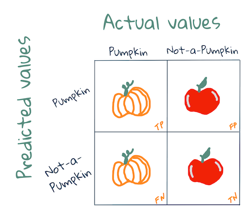
Every prediction lands in one of four boxes:
| Model says "Ghost" | Model says "Not Ghost" | |
|---|---|---|
| Really a ghost | ✅ True Positive | ❌ False Negative (missed it) |
| Really not | ❌ False Positive (false alarm) | ✅ True Negative |
The diagonal (the ✅ boxes) is where the model got it right. From this grid we compute accuracy — the share of predictions that were correct.
Warning: Accuracy alone can lie. If only 1 in 100 pumpkins is a ghost, a lazy model that always guesses "not ghost" scores 99% accuracy — while catching exactly zero ghosts! That's why the confusion matrix matters: it shows what kind of mistakes a model makes, not just how many.
Try This! Picture a smoke detector as a classifier. What would a false positive be (and why is it annoying)? What would a false negative be (and why is it dangerous)? This one example makes it clear why we care about the type of error, not just the total count.
Key Takeaway: Logistic regression predicts categories, not numbers. The sigmoid squashes any score into a 0–1 probability, with 0.5 as the usual cutoff. Categories must be encoded into numbers first (ordinal for ranked, one-hot for unordered), the code keeps the familiar fit/predict shape, and a confusion matrix reveals not just how often the model is right but what kind of mistakes it makes.
This module is adapted from Microsoft's open-source ML-For-Beginners curriculum (MIT License). Diagrams by Dasani Madipalli.