"Statistics is how we summarize a mountain of data into a few numbers that actually tell us something."
Learning Objectives
By the end of this module, you will be able to:
- Find the center of data (mean, median, mode)
- Describe how spread out data is
- Understand correlation
- Avoid a classic statistics trap
1. The Center of Data
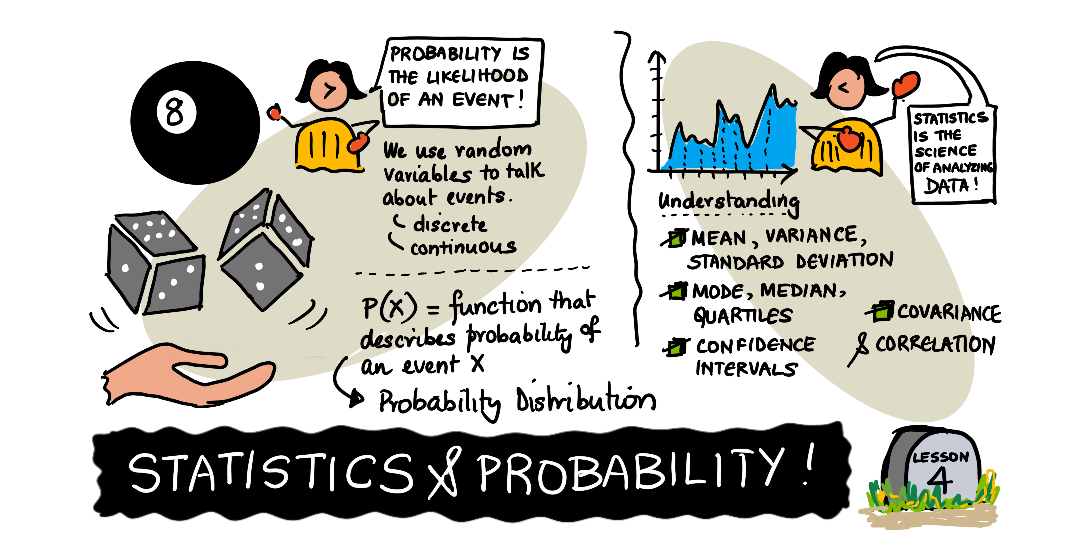
Three ways to describe a "typical" value:
| Measure | Meaning | Watch out |
|---|---|---|
| Mean | The average | Skewed by extreme values |
| Median | The middle value | Robust to outliers |
| Mode | The most common value | Good for categories |
Simple example: Five salaries: 30k, 32k, 35k, 38k, and 500k. The mean (~127k) is misleading; the median (35k) describes the typical person far better. One outlier wrecked the average.
Explain like I'm new: To find the median, line the values up smallest to largest and pick the one in the middle. With the salaries above, the middle value is 35k. Because it only cares about position, not size, that one giant 500k salary can't drag it around — which is exactly why the median is so trustworthy when a few extreme values exist.
The mean is easy to compute by hand: add every value and divide by how many there are. For the salaries that's (30 + 32 + 35 + 38 + 500) ÷ 5 = 127k. Notice how the single 500k value single-handedly pushed the "average" above what four of the five people actually earn. The mode — the most common value — is the odd one out: it works even on things that aren't numbers, like the most-ordered drink or the most common survey answer, where a mean makes no sense at all.
Real-world use case: House prices are almost always reported as a median, not a mean, for exactly this reason. A handful of multi-million-dollar mansions would drag the mean far above what a typical home costs. The median price answers the question people actually care about: "what does a normal house in this area cost?"
2. How Spread Out Is It?
The center isn't enough — we also need spread:
- Range — highest minus lowest
- Standard deviation — how far values typically sit from the mean (small = clustered, large = scattered)
Key idea: Two datasets can share the same average but feel completely different. "Average" temperature of 20°C could mean a steady spring day or freezing nights and scorching afternoons. Always look at spread, not just the center.
A concrete picture: imagine two classes that both average 70% on a test. In Class A everyone scored between 68 and 72 — tight, predictable, small standard deviation. In Class B, half scored 40 and half scored 100 — huge spread. Same average, wildly different reality. A teacher would help those two classes in completely different ways, and only the spread reveals that.
Data scientist tip: Report a center and a spread together — "average delivery time is 3 days, give or take 2" tells a far more honest story than "average is 3 days." The give-or-take is where the risk hides.
3. Correlation
Correlation measures whether two things move together, from -1 to +1:
- +1 — rise together
- 0 — no relationship
- -1 — one rises as the other falls
A value near +0.9 means a strong upward link (taller people tend to weigh more); near -0.9 means a strong opposite link (the more you exercise, the lower your resting heart rate); near 0 means the two barely track each other at all. The sign tells you the direction; the size tells you how tight the pattern is.
Common mistake: Treating correlation as proof of cause (Module 2). A strong correlation is a clue worth investigating, not a conclusion. Something else may be driving both.
Try this: Jot down your daily coffee cups and hours of sleep for a week, then eyeball whether they move together, opposite, or not at all. You've just estimated a correlation by hand — the same idea, only formalized with a number.
Key Takeaway: Statistics summarizes data. Describe its center with mean (average, sensitive to outliers), median (middle, robust), or mode (most common); describe its spread with range and standard deviation. Correlation (-1 to +1) shows whether things move together — but never mistake it for causation.
Further Learning
Adapted from Microsoft's Data Science for Beginners (MIT License). Sketchnote by Nitya Narasimhan.